Plotting FIDs and spectra from a DataArray

plot_fid/plot_spectra now take a chemical_shift/time-dimensioned xr.DataArray directly — how do I see that without loading a real scan?

xmris.simulate_fid() builds exactly the kind of DataArray MRSSeries/RawMRISeries produce from real data — time-dimensioned, with reference_frequency/carrier_ppm in .attrs — so it’s the fixture of choice here: fully synthetic, seeded, no scanner file needed.

Function	What it does here
`plot_fid()`	plots the simulated FID against its `time` coord
`plot_spectra()`	plots the phased spectrum against its `chemical_shift` coord

from loguru import logger
from matplotlib.pyplot import rcParams
from matplotlib_inline.backend_inline import set_matplotlib_formats

set_matplotlib_formats("retina")
rcParams["figure.dpi"] = 150
rcParams["figure.figsize"] = [6, 4]


logger.remove()

import matplotlib.pyplot as plt
import numpy as np
import xarray as xr
from xmris import simulate_fid

from mnutils.plotting.spectra import plot_fid, plot_spectra

1. Simulate 5 repetitions of a FID¶

Two peaks — a big one at 4.68 ppm (water), a smaller one at 3.0 ppm — damped, phased, with a touch of noise so the plot doesn’t look artificially perfect. Simulating 5 noisy repetitions and stacking them along a new average dim gives one dataset that covers both the single-spectrum case below and the multi-line case later on this page — the same data throughout, not two different fixtures:

fids = xr.concat(
    [
        simulate_fid(
            amplitudes=[1.0 * (seed + 1), 0.4 * (seed / 5 + 1)],
            chemical_shifts=[4.68, 3.0],
            reference_frequency=19.6,  # MHz, ~ 2H at 3T
            carrier_ppm=4.68,
            spectral_width=1000.0,
            n_points=700,
            dampings=[30.0, 20.0],
            target_snr=40.0,
            seed=seed,
        )
        for seed in range(5)
    ],
    dim="average",
)
fid = fids.isel(average=0)
fids

simulate_fid always returns a time-dimensioned DataArray — the same shape RawMRISeries.fids produces from a real scan — so everything below works identically against either source.

2. Plot the FID — `data=` is the whole call¶

No header, no dwelltime/deadtime: the time coord already carries the axis, in seconds, and plot_fid converts it to ms for display.

ax = plot_fid(data=fid)
plt.show()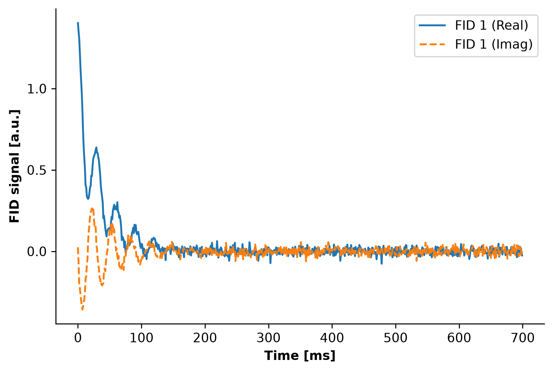

# STRICT TESTS: plot_fid read the axis from the DataArray's time coord, not from headers
np.testing.assert_allclose(
    ax.lines[0].get_xdata(),
    fid.coords["time"].values * 1e3,
    err_msg="plot_fid's x-axis should be the time coord converted to ms",
)
assert ax.get_xlabel() == "Time [ms]"

3. FFT, phase, plot — no phasing inside the plot call¶

plot_spectra only plots; phasing happens upstream through the xmr accessor, the same chain MRSSeries.phase_avg_spec uses on real data:

spectrum = fid.xmr.autophase().xmr.to_ppm()
ax = plot_spectra(data=spectrum)
plt.show()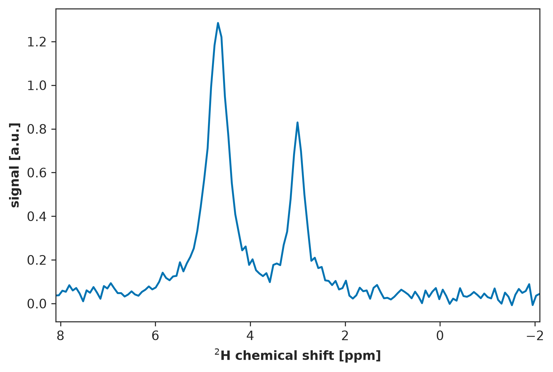

# STRICT TESTS: plot_spectra read ppm from the chemical_shift coord, and the water peak
# (the biggest simulated amplitude, at 4.68 ppm) is the tallest point on the line.
np.testing.assert_allclose(
    ax.lines[0].get_xdata(),
    spectrum.coords["chemical_shift"].values,
    err_msg="plot_spectra's x-axis should be the chemical_shift coord",
)
ppm_axis = ax.lines[0].get_xdata()
peak_ppm = ppm_axis[np.argmax(ax.lines[0].get_ydata())]
assert abs(peak_ppm - 4.68) < 0.2, (
    f"expected the water peak near 4.68 ppm, got {peak_ppm:.2f}"
)

4. Several FIDs and spectra at once, with custom labels¶

An extra dim beyond time/chemical_shift becomes one line per slice — no loop needed. The 5 repetitions simulated in step 1 are exactly that shape already; passing labels overrides the default "FID N"/"Spectrum N" naming:

labels = [f"Repetition {i + 1}" for i in range(fids.sizes["average"])]

ax_fid = plot_fid(data=fids, labels=labels)
plt.show()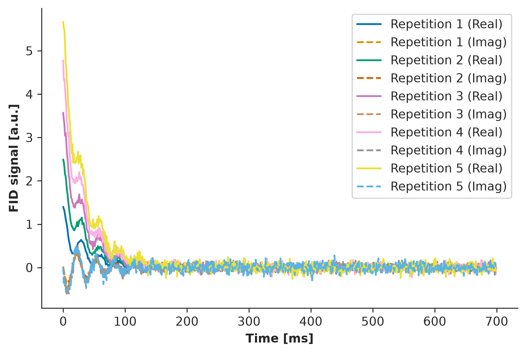

# STRICT TESTS: 5 repetitions -> 5 real + 5 imag lines, each labelled from `labels`
assert len(ax_fid.lines) == 10
assert [line.get_label() for line in ax_fid.lines[::2]] == [
    f"{label} (Real)" for label in labels
]

spectra = fids.xmr.to_spectrum().xmr.autophase().xmr.to_ppm()

ax_spectra = plot_spectra(data=spectra, labels=labels)
plt.show()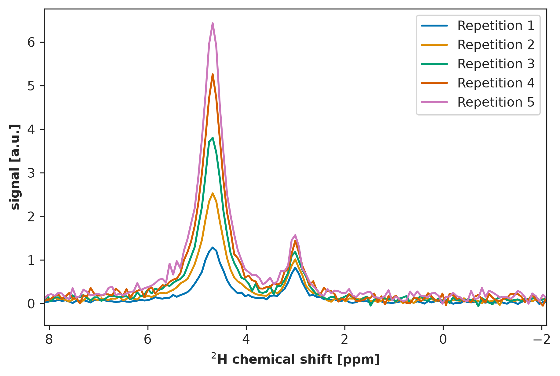

# STRICT TESTS: 5 repetitions -> 5 lines, each labelled from `labels`, water peak near 4.68 ppm
assert len(ax_spectra.lines) == 5
assert [line.get_label() for line in ax_spectra.lines] == labels
for line in ax_spectra.lines:
    ppm_axis = line.get_xdata()
    peak_ppm = ppm_axis[np.argmax(line.get_ydata())]
    assert abs(peak_ppm - 4.68) < 0.2, (
        f"expected the water peak near 4.68 ppm for {line.get_label()}, got {peak_ppm:.2f}"
    )

5. Manual arrays still work¶

Both functions keep the old array-based call as a fallback — for data with no DataArray to begin with. data takes priority whenever both are given:

ax = plot_spectra(
    ppm=spectrum.coords["chemical_shift"].values,
    spectra=spectrum.values.real,
)
plt.show()

Plotting FIDs and spectra from a DataArray

1. Simulate 5 repetitions of a FID¶

2. Plot the FID — data= is the whole call¶

3. FFT, phase, plot — no phasing inside the plot call¶

4. Several FIDs and spectra at once, with custom labels¶

5. Manual arrays still work¶

2. Plot the FID — `data=` is the whole call¶