The GESeries class hierarchy

A GE series folder can hold very different shapes of data depending on what was acquired: a 3D anatomical volume, a single-voxel spectrum averaged over time, a spectroscopic-imaging grid, or a dynamic wash-in series sampled every few seconds. GESeries isn’t one class trying to cover all of that — it’s a small hierarchy, and ExamBase picks the right subclass for a folder so you don’t have to guess it yourself.

The examples below load fixtures generated on the fly by mnutils.testing.build_fake_exam -- see the diary entry for why nothing here is a real scan.

from loguru import logger

logger.remove()

import numpy as np

from mnutils.GESeries import MRISeries, MRSISeries, MRSSeries, MRSWashinSeries, NiiBase
from mnutils.plotting.spectra import plot_fid, plot_spectra
from mnutils.testing import build_fake_exam
from mnutils.utils.nifti import get_display_affine, get_display_zooms

DATASETS = build_fake_exam("brain_mrs_mrsi_exam")
DATA_FOLDER = DATASETS / "data"

NiiBase — a NIfTI image, oriented and displayable¶

Every series that has a NIfTI ends up with a NiiBase (or subclass) wrapping it: nii, affine, and helpers like images()/display() that apply a display orientation consistently across the toolbox, so plotting code never re-derives it.

MRISeries — a NIfTI series, found by its sidecar¶

MRISeries is what you get for a series that has a NIfTI but no raw scanner exam data — typically an anatomical scan. It finds the NIfTI through the SeriesNumber in its JSON sidecar, whatever the folder is called. MNUtils never converts DICOMs: run dcm2niix -b y first, or the series logs a warning that spells out the command and loads without a NIfTI.

t1 = MRISeries(DATA_FOLDER, 2)  # 002_3D_Ax_T1_BRAVO
print(f"Data shape: {t1.nii.shape}")
print(f"Voxel size (mm): {t1.nii.header.get_zooms()}")  # thin in-plane, thick slices
display_plane = "axial"
print(f"Display affine:\n{get_display_affine(t1.nii, display_plane=display_plane)}")
print(f"Display zooms (mm): {get_display_zooms(t1.nii, display_plane=display_plane)}")
t1.display(cmap="gray")  # Axial is the default

Data shape: (188, 256, 186)
Voxel size (mm): (0.88, 0.88, 0.88)
Display affine:
[[  0.          -0.88         0.          81.43999636]
 [ -0.88         0.           0.         106.27999604]
 [  0.           0.           0.88       -77.12000275]
 [  0.           0.           0.           1.        ]]

Display zooms (mm): (0.8799999952316284, 0.8799999952316284)

display_plane = "coronal"
print(f"Display affine:\n{get_display_affine(t1.nii, display_plane=display_plane)}")
print(f"Display zooms (mm): {get_display_zooms(t1.nii, display_plane=display_plane)}")
t1.display(cmap="gray", display_plane=display_plane)

Display affine:
[[  0.          -0.88         0.          81.43999636]
 [  0.           0.          -0.88       106.27999604]
 [ -0.88         0.           0.          85.67999637]
 [  0.           0.           0.           1.        ]]
Display zooms (mm): (0.8799999952316284, 0.8799999952316284)

display_plane = "sagittal"
print(f"Display affine:\n{get_display_affine(t1.nii, display_plane=display_plane)}")
print(f"Display zooms (mm): {get_display_zooms(t1.nii, display_plane=display_plane)}")
t1.display(cmap="gray", display_plane=display_plane)

Display affine:
[[  0.           0.          -0.88        81.43999636]
 [  0.          -0.88         0.         106.27999604]
 [ -0.88         0.           0.          85.67999637]
 [  0.           0.           0.           1.        ]]
Display zooms (mm): (0.8799999952316284, 0.8799999952316284)

# STRICT TESTS: MRISeries
assert isinstance(t1, NiiBase)
assert t1.nii.ndim == 3

Anisotropic voxels: display()'s zooms correction¶

t1 above happens to look right in every plane, but only because it was acquired isotropically -- every voxel is a cube, so a square-pixel render matches real anatomy no matter which axis ends up in-plane. A real 2D-acquired scan usually isn’t a cube: thin in-plane pixels, thick slices. Reorient one of those to a different display_plane and the thick axis can land in-plane, where rendering it as square pixels stretches or squashes it relative to real anatomy.

NiiBase.display derives the physical (row, col) spacing of whichever two axes are currently in-plane (utils.nifti.get_display_zooms, built on the same reorientation images() applies) and passes it to display_images as zooms, so the render stays proportioned to real anatomy in every plane -- without resampling the underlying data.

pd = MRISeries(DATA_FOLDER, 4)  # 004_2D_Ax_PD
print(f"Data shape: {pd.nii.shape}")
print(f"Voxel size (mm): {pd.nii.header.get_zooms()}")  # thin in-plane, thick slices
display_plane = "axial"
print(f"Display affine:\n{get_display_affine(pd.nii, display_plane=display_plane)}")
print(f"Display zooms (mm): {get_display_zooms(pd.nii, display_plane=display_plane)}")
pd.display(cmap="gray")

Data shape: (191, 250, 54)
Voxel size (mm): (0.8578751, 0.8593749, 2.3999972)
Display affine:
[[ 5.19883633e-03 -8.57854128e-01  8.43399763e-03  8.08354541e+01]
 [-8.49813223e-01 -4.68388898e-03  3.56777370e-01  8.60981830e+01]
 [ 1.27732873e-01  3.75264464e-03  2.37331533e+00 -6.36348228e+01]
 [ 0.00000000e+00  0.00000000e+00  0.00000000e+00  1.00000000e+00]]
Display zooms (mm): (0.8593749056872297, 0.8578751225471344)

display_plane = "coronal"
print(f"Display affine:\n{get_display_affine(pd.nii, display_plane=display_plane)}")
print(f"Display zooms (mm): {get_display_zooms(pd.nii, display_plane=display_plane)}")
pd.display(cmap="gray", display_plane=display_plane)

Display affine:
[[-8.43399763e-03 -8.57854128e-01  5.19883633e-03  8.12824560e+01]
 [-3.56777370e-01 -4.68388898e-03 -8.49813223e-01  1.05007384e+02]
 [-2.37331533e+00  3.75264464e-03  1.27732873e-01  6.21508900e+01]
 [ 0.00000000e+00  0.00000000e+00  0.00000000e+00  1.00000000e+00]]
Display zooms (mm): (2.3999972708654984, 0.8578751225471344)

display_plane = "sagittal"
print(f"Display affine:\n{get_display_affine(pd.nii, display_plane=display_plane)}")
print(f"Display zooms (mm): {get_display_zooms(pd.nii, display_plane=display_plane)}")
pd.display(cmap="gray", display_plane=display_plane)

Display affine:
[[-8.43399763e-03  5.19883633e-03 -8.57854128e-01  8.12824560e+01]
 [-3.56777370e-01 -8.49813223e-01 -4.68388898e-03  1.05007384e+02]
 [-2.37331533e+00  1.27732873e-01  3.75264464e-03  6.21508900e+01]
 [ 0.00000000e+00  0.00000000e+00  0.00000000e+00  1.00000000e+00]]
Display zooms (mm): (2.3999972708654984, 0.8593749056872297)

# STRICT TESTS: anisotropic voxels
atol = 0.001
assert isinstance(pd, NiiBase)
axial_row_zoom, axial_col_zoom = get_display_zooms(pd, display_plane="axial")
# Row zoom should be around 0.859 and col zoom around 0.857
assert np.isclose(axial_row_zoom, 0.859, atol=atol)
assert np.isclose(axial_col_zoom, 0.857, atol=atol)
assert np.isclose(axial_row_zoom, axial_col_zoom, atol=0.1)  # Axial zooms should be equal
# Row zoom should be around 2.4 and col zoom around 0.857
coronal_row_zoom, coronal_col_zoom = get_display_zooms(pd, display_plane="coronal")
assert np.isclose(coronal_row_zoom, 2.4, atol=atol)
assert np.isclose(coronal_col_zoom, 0.857, atol=atol)
assert coronal_row_zoom != coronal_col_zoom

sag_row_zoom, sag_col_zoom = get_display_zooms(pd, display_plane="sagittal")
# Row zoom should be around 2.4 and col zoom around 0.859
assert np.isclose(sag_row_zoom, 2.4, atol=atol)
assert np.isclose(sag_col_zoom, 0.859, atol=atol)
assert sag_row_zoom != sag_col_zoom

# Test a local dataset. If env path not defined - skip this test. This is a local dataset and not part of the repo.
import os
from pathlib import Path

from dotenv import load_dotenv

load_dotenv()

LOCAL_TEST_DATASET_PATH = os.getenv("LOCAL_TEST_DATASET")
if LOCAL_TEST_DATASET_PATH is not None and Path(LOCAL_TEST_DATASET_PATH).exists():
    t1_patient = MRISeries(Path(LOCAL_TEST_DATASET_PATH), 2)
else:
    t1_patient = None

if t1_patient is not None:
    display_plane = "axial"
    print(f"Display affine:\n{get_display_affine(t1_patient.nii, display_plane=display_plane)}")
    print(f"Display zooms (mm): {get_display_zooms(t1_patient.nii, display_plane=display_plane)}")
    t1_patient.display(display_plane=display_plane, cmap="gray")

if t1_patient is not None:
    display_plane = "coronal"
    print(f"Display affine:\n{get_display_affine(t1_patient.nii, display_plane=display_plane)}")
    print(f"Display zooms (mm): {get_display_zooms(t1_patient.nii, display_plane=display_plane)}")
    t1_patient.display(display_plane=display_plane, cmap="gray")

if t1_patient is not None:
    display_plane = "sagittal"
    print(f"Display affine:\n{get_display_affine(t1_patient.nii, display_plane=display_plane)}")
    print(f"Display zooms (mm): {get_display_zooms(t1_patient.nii, display_plane=display_plane)}")
    t1_patient.display(display_plane=display_plane, cmap="gray")

MRSSeries — a single-voxel spectrum over time¶

A series with both raw exam data and a NIfTI (or no NIfTI at all, for a pure spectroscopy acquisition) loads as one of the RawMRISeries subclasses instead. MRSSeries holds a single-voxel spectrum with an averages dimension — one spectrum per repetition, not yet combined.

mrs = MRSSeries(DATA_FOLDER, 7)  # 006_MRS_unloc
mrs.spec

plot_spectra(mrs.avg_spec)

<Axes: xlabel='$^2$H chemical shift [ppm]', ylabel='signal [a.u.]'>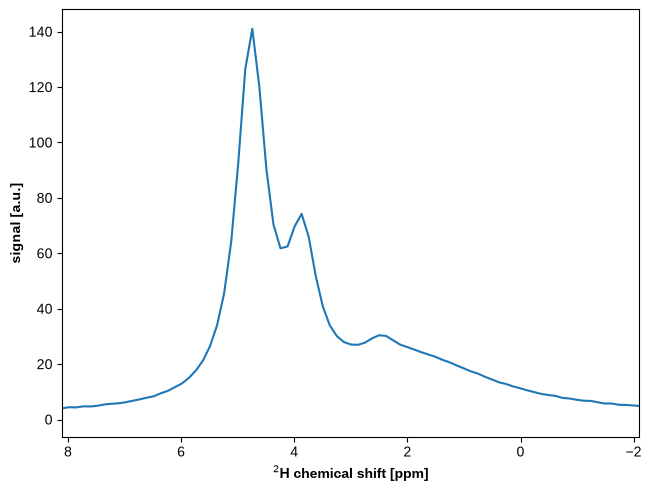

# STRICT TESTS: MRSSeries
assert mrs.spec.dims == ("averages", "chemical_shift")
assert mrs.spec.sizes["averages"] == mrs.averages
assert mrs.nucleus == 2

avg_fid/avg_spec collapse the averages dimension; see Loading a series and an exam for a worked example.

MRSWashinSeries — the same spectrum, resolved over time¶

A wash-in acquisition is structurally an MRSSeries — same averages × chemical_shift shape — but its averages are meant to be grouped into time bins and fit independently, tracking a metabolite as it washes in. MRSWashinSeries adds fit_grouped_by_duration() and plot_washin() on top of everything MRSSeries already gives you.

washin = MRSWashinSeries(DATA_FOLDER, 7)  # 007_MRS_washin
washin.spec

washin.plot_washin(group_duration=60)

<Axes: xlabel='$^2$H chemical shift [ppm]', ylabel='signal [a.u.]'>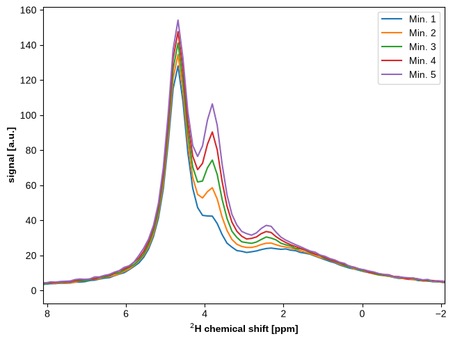

# STRICT TESTS: MRSWashinSeries
assert isinstance(washin, MRSSeries)
assert washin.spec.dims == ("averages", "chemical_shift")
assert washin.fit_results == []  # nothing fit yet

MRSISeries — a spectroscopic-imaging grid¶

MRSISeries is the spatial counterpart: a spectrum per voxel, laid out on a 3D grid (chemical_shift × i × j × k). It carries per-voxel fitting (fit_all_voxels, fit_single_voxel) and an SNR mask used to skip voxels with no real signal.

mrsi = MRSISeries(DATA_FOLDER, 8)  # 008_MRSI_pseudo_S700_X10_Y10_Z10_T1_C1
print(mrsi.spec.dims, mrsi.spec.shape)
print(mrsi.dims)  # spatial grid (i, j, k)
mrsi.spec

('chemical_shift', 'i', 'j', 'k') (700, 16, 16, 16)
(16, 16, 16)

from mnutils.plotting.images import inspect_MRSI_spectra

inspect_MRSI_spectra(t1, mrsi)

# STRICT TESTS: MRSISeries
assert mrsi.spec.dims == ("chemical_shift", "i", "j", "k")
assert mrsi.dims == mrsi.spec.shape[1:4]
assert isinstance(mrsi, NiiBase)  # create_MRSI_nii() gives it a displayable volume too

NiiBase operations: resampling and overlays¶

Two NiiBase images at different resolutions come up constantly — an anatomical scan and an MRSI grid, say — and need to be compared voxel-for-voxel. resample_self_to reslices one onto another’s grid; overlay_nifti_data_on_T1 (from mnutils.plotting.images) plots the result on top of an anatomical volume. These examples use the fake 20250408-NIST-Mag2 exam, a phantom scan where series 2 is the anatomical T1 and series 5 is an MRSI grid.

resampled = mrsi.resample_self_to(t1.nii, order=0)
print(isinstance(resampled, NiiBase), resampled.nii.shape == t1.nii.shape)

True True

# STRICT TESTS: resample_self_to
assert isinstance(resampled, NiiBase)
assert resampled.nii.shape == t1.nii.shape

images() applies the display orientation and returns a plain array — what display() and the overlay helpers plot under the hood:

from mnutils.plotting.images import overlay_nifti_data_on_T1

overlay_nifti_data_on_T1(t1.nii, mrsi.nii)

overlay_nifti_data_on_T1(t1.nii, mrsi.RAW_exp.nii)

MRSISeries carries a few more properties worth knowing about beyond spec: an SNR-based mask for skipping low-signal voxels, a computed voxel size, and per-voxel spectrum access.

print(mrsi.voxel_size)  # mm, derived from field_of_view / matrix size
print(mrsi.SNR_map.dims)
voxel_spectrum = mrsi.get_voxel_spectrum(10, 10, 8)
plot_spectra(voxel_spectrum)

10.339999943971634

('i', 'j', 'k')

/home/runner/work/mnutils/mnutils/.venv/lib/python3.12/site-packages/pyAMARES/kernel/fid.py:357: RuntimeWarning: invalid value encountered in scalar divide
  return signal_p / noise_p

<Axes: xlabel='$^2$H chemical shift [ppm]', ylabel='signal [a.u.]'>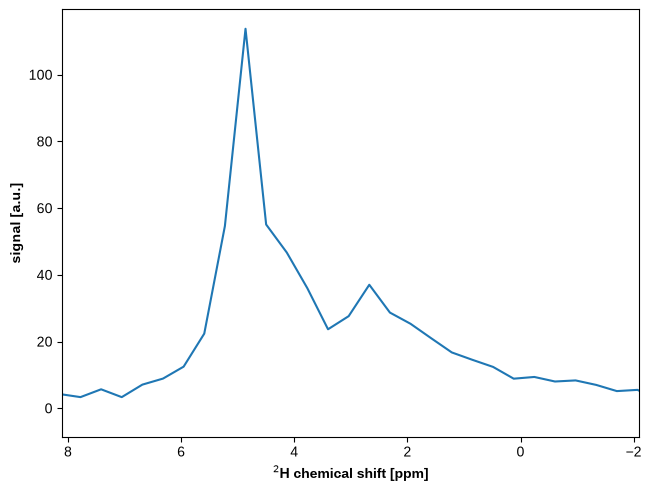

# STRICT TESTS: MRSISeries extras
assert mrsi.SNR_map.dims == ("i", "j", "k")
assert mrsi.create_MRSI_affine().shape == (4, 4)
assert voxel_spectrum.dims == ("chemical_shift",)

A bounded panel_height keeps a three-panel overlay on one row¶

overlay_nifti_data_on_T1 lays out three panels -- T1, data, overlay -- in a CSS grid whose per-panel width cap is derived from panel_height times the frame’s aspect ratio. Bound that height down far enough and the cap used to fall under the grid’s fixed column floor (grid.panel_min_width, 9rem by default): the widget then constrained itself narrower than its own three columns needed, and auto-fit dropped one onto a second row. t1’s axial frame (aspect ≈0.73) only needs panel_height bounded below ~12rem to hit that:

overlay_nifti_data_on_T1(t1.nii, mrsi.nii, panel_height="10rem")

All three panels stay on one row -- the width cap is now clamped up to the column floor instead of falling below it (--mnu-panel-w-cap in image_grid.css).