How much of this MRSI voxel is inside the mask?
I have a segmentation at sub-millimetre resolution and a spectroscopic grid at ten-plus millimetres, on a different field of view. What fraction of each spectrum’s voxel does the segmentation actually cover?
mask_occupancy() answers that in one call. This
page takes the call apart and rebuilds it by hand on the synthetic brain exam, one step at a time,
checking each step against the library as it goes — so the number it returns is something you can
audit rather than trust.
import nibabel as nib
import numpy as np

from mnutils.GESeries import MRISeries, MRSISeries, NiiBase
from mnutils.testing import build_fake_exam
from mnutils.utils.partial_volume import mask_occupancy, target_halfwidths

root = build_fake_exam("brain_mrs_mrsi_exam")
t1 = MRISeries(root / "data", 2)
mrsi = MRSISeries(root / "data", 8)

# Segmentations of that same T1, written beside the exam by the fixture builder.
brain_mask: nib.Nifti1Image = nib.load(root / "derived" / "brain_mask.nii.gz")  # ty:ignore[invalid-assignment]
tissue_seg: nib.Nifti1Image = nib.load(root / "derived" / "tissue_seg.nii.gz")  # ty:ignore[invalid-assignment]
That is four volumes but only two grids, and the split between them is the whole problem. Look at
each one before any arithmetic happens — display() draws an
interactive grid with a slice slider rather than a static figure, so scrub through a volume instead
of trusting whichever slice a figure happened to pick.
The T1 is the fine grid, and the anatomy every other volume on this page is defined against:
t1.display(cmap="gray")The same head, as the spectroscopic acquisition sees it. One voxel per spectrum, a couple of dozen across the brain — each of those blocks is what the rest of this page has to attach a fraction to:
mrsi.RAW_exp.display()Back on the fine grid, brain_mask is that T1 reduced to a binary in-or-out. This is the mask in
“how much of this MRSI voxel is inside the mask”: everything below is about pushing it onto the
blocky grid above without losing or inventing volume. A bare nibabel image gets wrapped in
NiiBase to borrow the same viewer:
NiiBase(brain_mask).display(cmap="viridis_r")tissue_seg divides that same interior further into three categories. A single mask is the easier
story, so most of the page uses brain_mask; the segmentation returns at the end, where the
per-label fractions have to add back up to the whole voxel:
NiiBase(tissue_seg).display(cmap="okabe_ito", colorbar=True)Fine grid and blocky grid, side by side as numbers — this is the mismatch to reconcile:
target = mrsi.RAW_exp  # the blocky MRSI grid, one voxel per spectrum

print(f"mask   {brain_mask.shape}  voxel {np.abs(np.diag(brain_mask.affine)[:3]).round(2)} mm")
print(f"target {target.nii.shape}  voxel {np.abs(np.diag(target.nii.affine)[:3]).round(2)} mm")
mask (188, 256, 186) voxel [0.88 0.88 0.88] mm
target (16, 16, 16) voxel [10.34 14.08 10.23] mm
Anisotropic target voxels, a mask an order of magnitude finer, and two different fields of view. Nothing below special-cases any of that — it all lives in one matrix.
Step 1 — one matrix absorbs every difference between the grids
Both images carry an affine mapping their own voxel indices to world millimetres. Composing one with the inverse of the other gives a single transform from mask index to target index, and it absorbs the differing voxel size, field of view, position and obliquity at once:
A_mask = np.asarray(brain_mask.affine)
A_target = np.asarray(target.nii.affine)

tgt_from_mask = np.linalg.inv(A_target) @ A_mask
print(tgt_from_mask.round(4))
[[ 0.0851 0. 0. -0.4574]
[ 0. 0.0625 0. -0.4688]
[ 0. 0. 0.086 -0.457 ]
[ 0. 0. 0. 1. ]]
Read the diagonal as “how many mask voxels fit along one target voxel” (inverted): about 11.8, 16.0 and 11.6 respectively. Those non-integer ratios matter later.
The matrix is easier to believe when you draw it. Push every T1 voxel of one slice through
tgt_from_mask, take the target voxel each lands in, and colour it as a checkerboard: that is
the MRSI lattice, rendered on the anatomy by the same arithmetic the algorithm uses. Anything
mapping off the target grid is hatched — that is the overhang which will come back as low
coverage:
t1_data = np.asarray(t1.nii.dataobj)
z = t1_data.shape[2] // 2

slice_idx = np.indices(t1_data.shape[:2], dtype=np.float64)
slice_idx = np.stack([slice_idx[0], slice_idx[1], np.full(t1_data.shape[:2], float(z))])
slice_tgt = (
    np.einsum("ab,bij->aij", tgt_from_mask[:3, :3], slice_idx) + tgt_from_mask[:3, 3, None, None]
)
slice_bins = np.floor(slice_tgt + 0.5).astype(int)

on_grid = np.ones(slice_bins.shape[1:], dtype=bool)
for axis in range(3):
    on_grid &= (slice_bins[axis] >= 0) & (slice_bins[axis] < target.nii.shape[axis])

checker = np.where(on_grid, (slice_bins[0] + slice_bins[1]) % 2, np.nan)

fig, ax = plt.subplots(figsize=(4.2, 4.2), layout="constrained")
panel(ax, t1_data[:, :, z], "MRSI voxel lattice over the T1", cmap="gray")
ax.imshow(checker.T, origin="lower", cmap="cool", alpha=0.35, interpolation="nearest")
off_grid = np.where(on_grid, np.nan, 1.0)
ax.imshow(off_grid.T, origin="lower", cmap="autumn", alpha=0.5, interpolation="nearest")
print(f"{100 * (~on_grid).mean():.1f}% of this T1 slice maps off the MRSI grid (shown in red)")
0.0% of this T1 slice maps off the MRSI grid (shown in red)
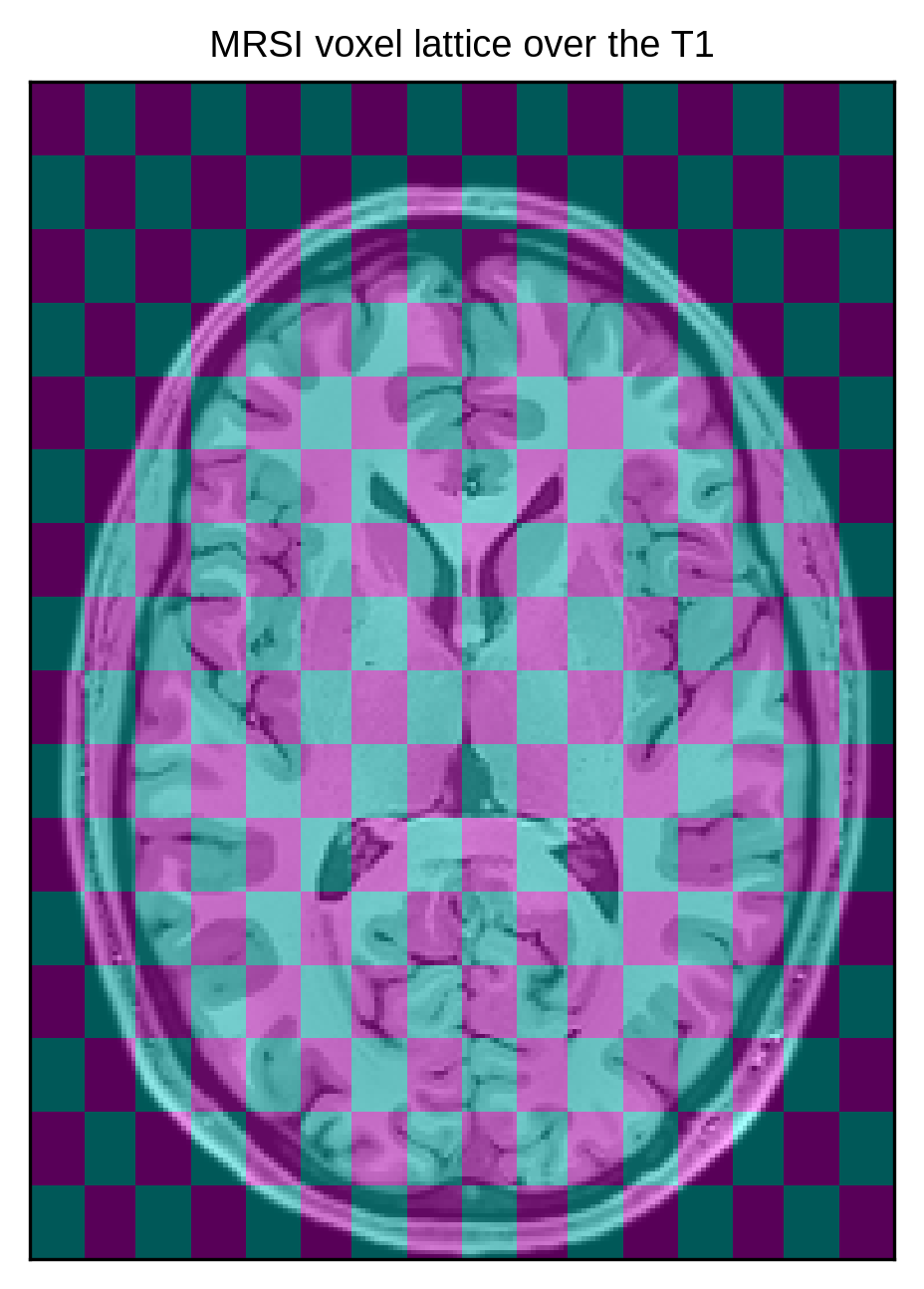
Each check is one MRSI voxel. They are visibly wider than they are tall — that is the anisotropy from the printout above — and the brain does not sit neatly inside them.
Step 2 — a voxel index names a centre, so the bin is floor(x + 0.5)
Map a mask voxel through tgt_from_mask and you get a fractional target coordinate. Turning that
into a bin is where the half-voxel bugs live: a NIfTI index names the centre of its voxel, so
target voxel n spans [n - 0.5, n + 0.5) and the bin is floor(x + 0.5) — not floor(x).
mask_idx = np.array([[94.0, 128.0, 93.0]])  # roughly the middle of the mask grid
mapped = mask_idx @ tgt_from_mask[:3, :3].T + tgt_from_mask[:3, 3]

print(f"mapped to target coordinate {mapped[0].round(3)}")
print(f"correct bin  floor(x + 0.5) = {np.floor(mapped + 0.5)[0].astype(int)}")
print(f"wrong bin    floor(x)       = {np.floor(mapped)[0].astype(int)}")
mapped to target coordinate [7.543 7.531 7.543]
correct bin floor(x + 0.5) = [8 8 8]
wrong bin floor(x) = [7 7 7]
Step 3 — one mask voxel is a box, and boxes straddle bins
Dropping each mask voxel whole into its nearest bin is the obvious thing to do, and it is wrong here in a way that is worth seeing rather than being told.
A mask voxel is not a point: it is a box. Under tgt_from_mask its half-extent along each target
axis is half the sum of the absolute values in that row — a sum, not just the diagonal, because an
oblique transform tilts the box across all three axes:
half = target_halfwidths(tgt_from_mask)
print(f"one mask voxel spans {(2 * half).round(4)} of a target voxel, per axis")
one mask voxel spans [0.0851 0.0625 0.086 ] of a target voxel, per axis
In one dimension the whole argument fits in a picture. A mask voxel is the shaded box; the target bins are the cells between the dashed edges. Nearest-bin gives the entire box to whichever bin holds its centre. Splitting gives each bin the share it actually covers:
# The real box is ~0.085 of a target voxel -- too thin to see. Drawn 4x wider here; the
# arithmetic below is the same either way.
draw_width = 4 * 2 * half[0]
centre = 3.5 - 0.35 * draw_width  # placed so it straddles the edge at 3.5
lo, hi = centre - draw_width / 2, centre + draw_width / 2
left = (min(hi, 3.5) - lo) / draw_width
right = 1.0 - left

fig, ax = plt.subplots(figsize=(7, 2.0), layout="constrained")
for edge in np.arange(2.5, 5.6, 1.0):
    ax.axvline(edge, color="0.4", ls="--", lw=1)
for n in (3, 4, 5):
    ax.text(n, 0.80, f"bin {n}", ha="center", fontsize=9, color="0.35")

ax.axvspan(lo, hi, ymin=0.2, ymax=0.6, color="tab:blue", alpha=0.5)
ax.plot([centre], [0.4], "o", color="tab:blue", ms=6)
ax.annotate(
    "nearest bin: all of it to bin 3",
    xy=(centre, 0.4),
    xytext=(2.60, 0.06),
    fontsize=8,
    color="tab:red",
    arrowprops={"arrowstyle": "->", "color": "tab:red"},
)
ax.text(
    3.62,
    0.66,
    f"split: {left:.2f} to bin 3, {right:.2f} to bin 4",
    ha="left",
    fontsize=9,
    color="tab:blue",
)
ax.set_xlim(2.5, 5.5)
ax.set_ylim(0, 0.95)
ax.set_yticks([])
ax.set_xlabel("target index")
print(f"drawn {draw_width:.3f} wide; the true box is {2 * half[0]:.3f} of a target voxel")
drawn 0.340 wide; the true box is 0.085 of a target voxel
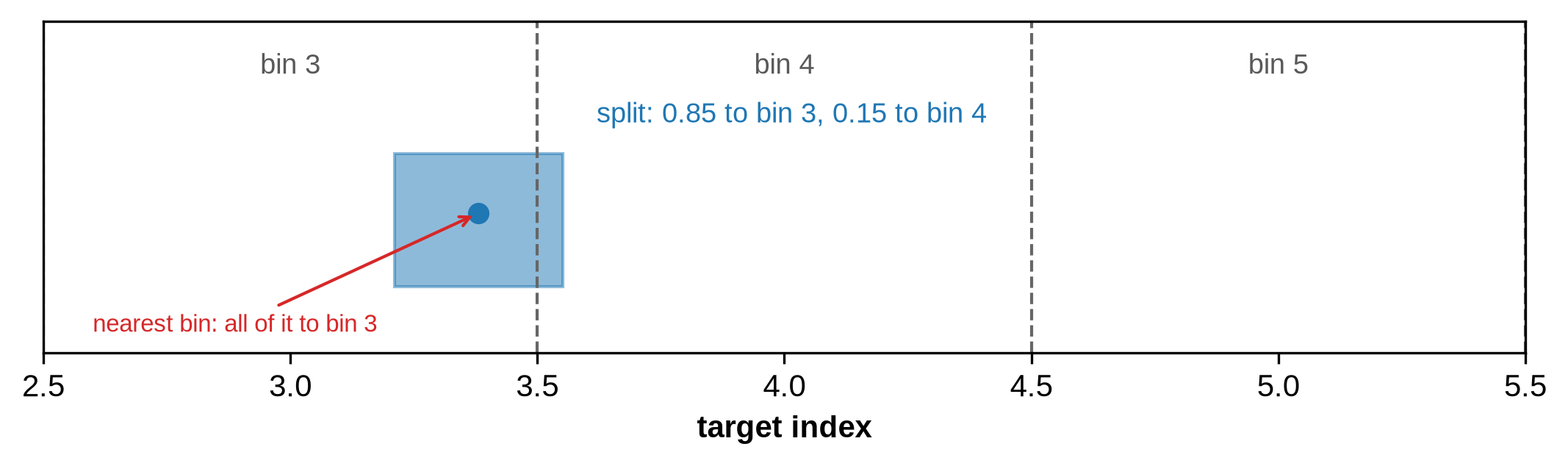
The box is well under one target voxel wide, so it reaches at most two bins per axis — eight combinations in 3-D, which is exactly what the implementation loops over.
Now the failure. Take a mask that is 1 everywhere, so every target voxel sitting fully
inside the mask’s field of view must come out at exactly 100 % coverage. Assign each mask voxel to
its nearest bin only, and count:
ones = np.ones(brain_mask.shape, dtype=np.float32)

idx = np.indices(brain_mask.shape, dtype=np.float64)
coords = (
    np.einsum("ab,bijk->aijk", tgt_from_mask[:3, :3], idx) + tgt_from_mask[:3, 3, None, None, None]
)
nearest = np.floor(coords + 0.5).astype(int)

inside = np.ones(nearest.shape[1:], dtype=bool)
for axis in range(3):
    inside &= (nearest[axis] >= 0) & (nearest[axis] < target.nii.shape[axis])

flat = np.ravel_multi_index(tuple(nearest[a][inside] for a in range(3)), target.nii.shape)
counts = np.bincount(flat, minlength=int(np.prod(target.nii.shape))).reshape(target.nii.shape)

nominal = 1.0 / abs(np.linalg.det(tgt_from_mask))  # mask voxels a full target voxel holds
print(f"a full target voxel should hold {nominal:.1f} mask voxels")
a full target voxel should hold 2185.5 mask voxels
Restrict to target voxels whose eight corners all fall inside the mask grid — those are provably 100 % covered — and look at what nearest-bin counting reports for them:
from nibabel import affines

corners = np.array(np.meshgrid([-0.5, 0.5], [-0.5, 0.5], [-0.5, 0.5])).reshape(3, -1).T
mask_from_tgt = np.linalg.inv(tgt_from_mask)
all_idx = np.indices(target.nii.shape).reshape(3, -1).T

interior = np.ones(len(all_idx), dtype=bool)
for corner in corners:
    p = affines.apply_affine(mask_from_tgt, all_idx + corner)
    interior &= np.all((p >= -0.5) & (p <= np.array(brain_mask.shape) - 0.5), axis=1)

nearest_coverage = (counts.reshape(-1) / nominal)[interior]
print(f"{interior.sum()} fully-interior target voxels")
print(f"nearest-bin coverage spans {nearest_coverage.min():.3f} to {nearest_coverage.max():.3f}")
print(
    f"that is a spread of {(nearest_coverage.max() - nearest_coverage.min()) * 100:.1f} points on voxels that are 100% covered"
)
3375 fully-interior target voxels
nearest-bin coverage spans 0.886 to 1.054
that is a spread of 16.8 points on voxels that are 100% covered
Those ratios from step 1 are the cause: at 11.75 mask voxels per target voxel, a target voxel
catches either 11 or 12 of them along that axis depending on where the lattice happens to fall.
The count quantises, so the fraction wobbles by roughly ±8 % — enough that a min_coverage=0.9
threshold would throw away hundreds of completely covered voxels.
The fix is to stop pretending the box is a point. Split each mask voxel between the bins it overlaps, in proportion to how much of it lands in each, separably per axis:
lower, upper = coords.reshape(3, -1) - half[:, None], coords.reshape(3, -1) + half[:, None]
first = np.floor(lower + 0.5)

total = np.zeros(int(np.prod(target.nii.shape)))
for si in (0.0, 1.0):
    for sj in (0.0, 1.0):
        for sk in (0.0, 1.0):
            bins = np.stack([first[0] + si, first[1] + sj, first[2] + sk])
            w = np.ones(bins.shape[1])
            for axis in range(3):
                n = bins[axis]
                overlap = np.minimum(upper[axis], n + 0.5) - np.maximum(lower[axis], n - 0.5)
                w *= np.clip(overlap, 0.0, None) / (2 * half[axis])
            keep = w > 0
            for axis in range(3):
                keep &= (bins[axis] >= 0) & (bins[axis] < target.nii.shape[axis])
            b = bins[:, keep].astype(int)
            total += np.bincount(
                np.ravel_multi_index((b[0], b[1], b[2]), target.nii.shape),
                weights=w[keep],
                minlength=total.size,
            )

split_coverage = (total / nominal)[interior]
print(f"overlap-split coverage spans {split_coverage.min():.6f} to {split_coverage.max():.6f}")
overlap-split coverage spans 1.000000 to 1.000000
Exactly 1.0 everywhere it should be. The weights of one mask voxel sum to 1 by construction, so nothing is created or lost — the mass simply lands in the right proportions.
Side by side on a mid-grid slice, with the same colour scale, the difference is not subtle. Both maps should be a flat field of 1.0 across the interior:
nearest_map = (counts / nominal).astype(float)
split_map = (total / nominal).reshape(target.nii.shape)
interior_map = interior.reshape(target.nii.shape)
k = target.nii.shape[2] // 2

fig, axes = plt.subplots(1, 3, figsize=(11, 3.3), layout="constrained")
h0 = panel(axes[0], nearest_map[:, :, k], "nearest bin", cmap="RdBu_r", vmin=0.85, vmax=1.15)
panel(axes[1], split_map[:, :, k], "overlap split", cmap="RdBu_r", vmin=0.85, vmax=1.15)
fig.colorbar(h0, ax=axes[:2], fraction=0.046, label="coverage")

axes[2].hist(nearest_map[interior_map], bins=40, alpha=0.7, label="nearest bin")
axes[2].hist(split_map[interior_map], bins=40, alpha=0.9, label="overlap split")
axes[2].axvline(1.0, color="k", ls="--", lw=1)
axes[2].set_title("coverage on fully-interior voxels", fontsize=9)
axes[2].set_xlabel("coverage")
axes[2].legend(fontsize=8)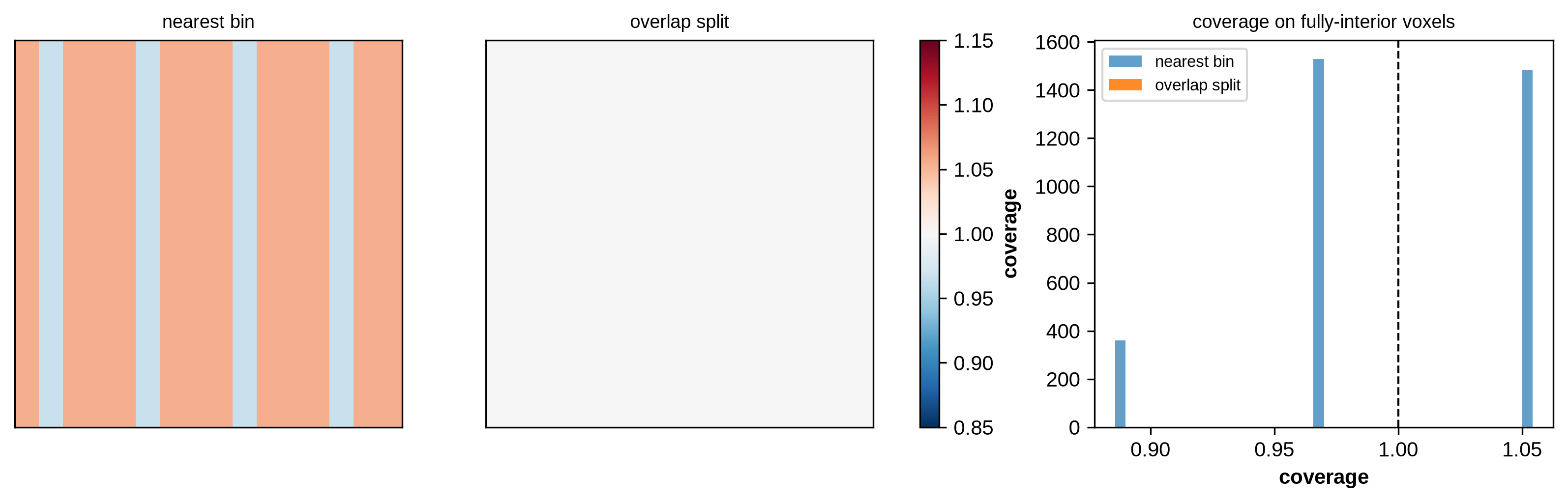
The left panel is the lattice beating against the anatomy grid; the middle panel is the constant it should have been all along. The histogram is the same story in one dimension — a smear across 0.89–1.05 collapsing to a single spike at 1.0.
Step 4 — the denominator is a determinant, not a ratio of voxel sizes
Turning a weighted count into a fraction needs to know how many mask voxels a full target voxel
holds. That is the ratio of the two voxel volumes, which is exactly 1 / |det(tgt_from_mask)| —
and unlike a per-axis ratio it stays correct for anisotropic and oblique grids, where “voxel size”
is not a single number per axis:
mask_voxel_mm3 = abs(np.linalg.det(A_mask[:3, :3]))
target_voxel_mm3 = abs(np.linalg.det(A_target[:3, :3]))

print(f"mask voxel   {mask_voxel_mm3:.4f} mm^3")
print(f"target voxel {target_voxel_mm3:.1f} mm^3")
print(f"ratio {target_voxel_mm3 / mask_voxel_mm3:.3f}  ==  1/|det| {nominal:.3f}")
mask voxel 0.6815 mm^3
target voxel 1489.4 mm^3
ratio 2185.500 == 1/|det| 2185.500
The call, and why it returns two arrays
Everything above is what one call does internally:
pv = mask_occupancy(brain_mask, target)
pvoccupancy and coverage answer different questions, and collapsing them into one number loses
the difference between no brain here and no anatomy here:
| Variable | Answers | Masked by min_coverage |
|---|---|---|
occupancy | how much of this voxel is inside the mask | yes — NaN below the threshold |
coverage | how much of this voxel the mask grid reached at all | no — always readable |
The MRSI grid overhangs the T1’s field of view, so some voxels genuinely have no anatomy to
measure against. Those come back NaN in occupancy and are explained by coverage:
n_nan = int(np.isnan(pv.occupancy).sum())
print(f"{n_nan} of {pv.occupancy.size} voxels are NaN (coverage < {pv.attrs['min_coverage']})")
print(
    f"every one of them has low coverage: {bool((pv.coverage.values[np.isnan(pv.occupancy.values[0])] < 0.9).all())}"
)
0 of 4096 voxels are NaN (coverage < 0.9)
every one of them has low coverage: True
The result carries world coordinates as 3-D x/y/z coordinates rather than one array per
axis. For an oblique acquisition world x depends on all three indices, so per-axis coordinates
would be quietly wrong exactly when obliquity matters:
print(pv.x.dims, pv.x.shape)
print(
    f"voxel (0,0,0) sits at ({float(pv.x[0, 0, 0]):.1f}, {float(pv.y[0, 0, 0]):.1f}, {float(pv.z[0, 0, 0]):.1f}) mm"
)
('i', 'j', 'k') (16, 16, 16)
voxel (0,0,0) sits at (-78.4, -111.5, -72.4) mm
Both affines travel with the result in .attrs, flattened row-major rather than nested — netCDF
attributes must be one-dimensional, and a nested 4×4 would make the whole Dataset impossible to
save. Reshape to get one back:
recovered = np.asarray(pv.attrs["target_affine"]).reshape(4, 4)
print(np.allclose(recovered, A_target))
True
Verifying it: three properties that must hold
Mass is conserved. The split only repartitions volume, so for a mask that lands entirely on the target grid, volume in must equal volume out as an identity rather than a tolerance. A sphere well inside both fields of view shows it cleanly:
sphere_idx = np.indices(brain_mask.shape)
centre = np.array(brain_mask.shape) // 2
sphere = (((sphere_idx - centre[:, None, None, None]) ** 2).sum(0) < 40**2).astype(np.float32)

pv_sphere = mask_occupancy(sphere, target, mask_affine=A_mask, min_coverage=0.0)
sphere_in = sphere.sum() * mask_voxel_mm3
sphere_out = float(pv_sphere.occupancy.sum()) * target_voxel_mm3
print(f"sphere in  {sphere_in / 1000:.3f} mL")
print(f"sphere out {sphere_out / 1000:.3f} mL")
print(f"relative error {abs(sphere_out - sphere_in) / sphere_in:.1e}")
sphere in 182.451 mL
sphere out 182.451 mL
relative error 3.4e-08
The brain mask is a different story, and the difference is worth knowing about: the MRSI grid here spans almost exactly the same extent as the T1, so the outermost rim of the brain maps off the target grid and is dropped. Conservation becomes an upper bound, and the shortfall tells you how much mask never made it onto the grid at all:
pv_full = mask_occupancy(brain_mask, target, min_coverage=0.0)

volume_in = brain_mask.get_fdata().sum() * mask_voxel_mm3
volume_out = float(pv_full.occupancy.sum()) * target_voxel_mm3
print(f"mask volume in {volume_in / 1000:.2f} mL")
print(f"volume out     {volume_out / 1000:.2f} mL")
print(f"lost off the edge of the MRSI grid: {(1 - volume_out / volume_in) * 100:.2f}%")
mask volume in 2699.25 mL
volume out 2699.25 mL
lost off the edge of the MRSI grid: 0.00%
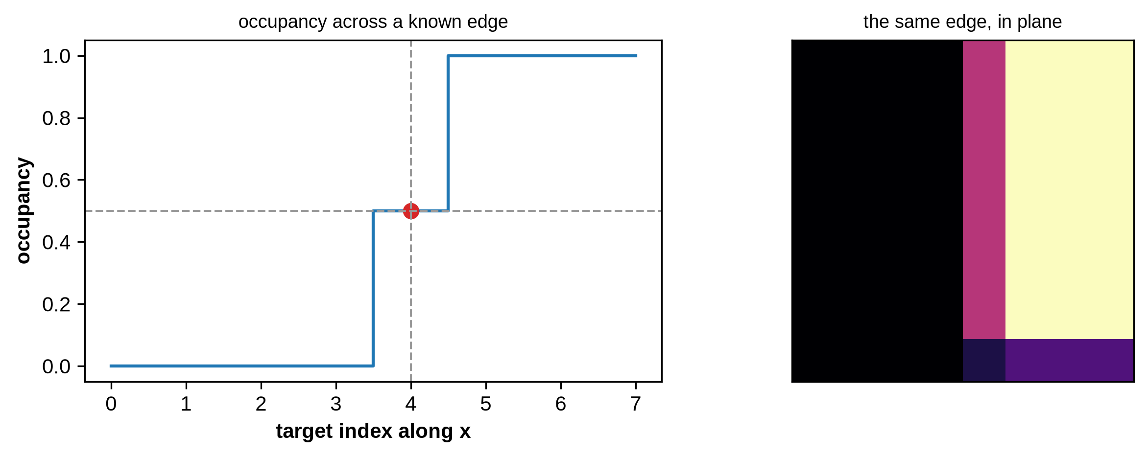
A known edge lands where geometry says. A half-space mask has an analytically exact answer, so the occupancy of the straddling voxel can be predicted rather than eyeballed.
The mask’s region is the union of its voxel boxes, not the set of its centres, so where that region begins depends on the grid’s phase. Offsetting the mask affine by half a voxel puts a voxel boundary exactly on world zero, which makes the expected answer a clean 0.5. Without that offset the region would start half a mask voxel early and the voxel would read 0.53125 — correct, but a worse thing to assert against:
n, vs, tn, tvs = 120, 0.5, 8, 8.0
edge_affine = np.diag([vs, vs, vs, 1.0])
edge_affine[:3, 3] = -vs * n / 2 + vs / 2  # a voxel boundary, not a centre, sits at world 0
grid_affine = np.diag([tvs, tvs, tvs, 1.0])
grid_affine[:3, 3] = -tvs * tn / 2

world_x = edge_affine[0, 0] * np.indices((n, n, n))[0] + edge_affine[0, 3]
half_space = nib.Nifti1Image((world_x >= 0).astype(np.float32), edge_affine)

edge = mask_occupancy(half_space, np.zeros((tn,) * 3), target_affine=grid_affine, min_coverage=0.0)
profile = edge.occupancy.values[0, :, tn // 2, tn // 2]
print(f"occupancy along x: {profile.round(3)}")
print(f"the voxel centred on the edge reads {profile[tn // 2]:.4f} (expected 0.5)")
occupancy along x: [0. 0. 0. 0. 0.5 1. 1. 1. ]
the voxel centred on the edge reads 0.5000 (expected 0.5)
A hard 0-to-1 step with exactly one half-valued voxel on the boundary, and no smearing into its neighbours — which is what a correctly centred, volume-conserving split looks like:
fig, axes = plt.subplots(1, 2, figsize=(8.5, 3.0), layout="constrained")

axes[0].step(np.arange(tn), profile, where="mid", color="tab:blue")
axes[0].plot([tn // 2], [profile[tn // 2]], "o", color="tab:red", ms=7)
axes[0].axhline(0.5, color="0.6", ls="--", lw=1)
axes[0].axvline(tn // 2, color="0.6", ls="--", lw=1)
axes[0].set_xlabel("target index along x")
axes[0].set_ylabel("occupancy")
axes[0].set_title("occupancy across a known edge", fontsize=9)

panel(
    axes[1],
    edge.occupancy.values[0, :, :, tn // 2],
    "the same edge, in plane",
    cmap="magma",
    vmin=0,
    vmax=1,
)
Labels partition the voxel. With the background counted as a label, the per-label occupancies must sum to the coverage exactly — there is nowhere else for the volume to go:
pv_seg = mask_occupancy(
    tissue_seg, target, labels={0: "background", 1: "csf", 2: "gm", 3: "wm"}, min_coverage=0.0
)
residual = np.abs(pv_seg.occupancy.sum("label").values - pv_seg.coverage.values).max()
print(f"labels present: {pv_seg.label.values.tolist()}")
print(f"max |sum(labels) - coverage| = {residual:.2e}")
labels present: ['background', 'csf', 'gm', 'wm']
max |sum(labels) - coverage| = 1.19e-07
Left to auto-detect, mask_occupancy finds the non-zero labels itself and the sum then falls
short of coverage by exactly the background fraction:
pv_auto = mask_occupancy(tissue_seg, target, min_coverage=0.0)
shortfall = (pv_auto.coverage.values - pv_auto.occupancy.sum("label").values).max()
print(f"auto-detected labels: {pv_auto.label.values.tolist()}")
print(f"largest shortfall vs coverage (the background): {shortfall:.3f}")
auto-detected labels: ['1', '2', '3']
largest shortfall vs coverage (the background): 1.000
Each label gets its own map, and they add up. The rightmost panel is the sum of the three tissue maps — every voxel’s remaining share is background:
k_seg = target.nii.shape[2] // 2
names = ["csf", "gm", "wm"]

fig, axes = plt.subplots(1, 4, figsize=(12, 3.1), layout="constrained")
for ax, label, name in zip(axes[:3], pv_auto.label.values, names, strict=True):
    handle = panel(
        ax,
        pv_auto.occupancy.sel(label=label).values[:, :, k_seg],
        f"label {label} ({name})",
        cmap="magma",
        vmin=0,
        vmax=1,
    )
total_tissue = pv_auto.occupancy.sum("label").values[:, :, k_seg]
panel(axes[3], total_tissue, "sum of all three", cmap="magma", vmin=0, vmax=1)
fig.colorbar(handle, ax=axes, fraction=0.03, label="occupancy")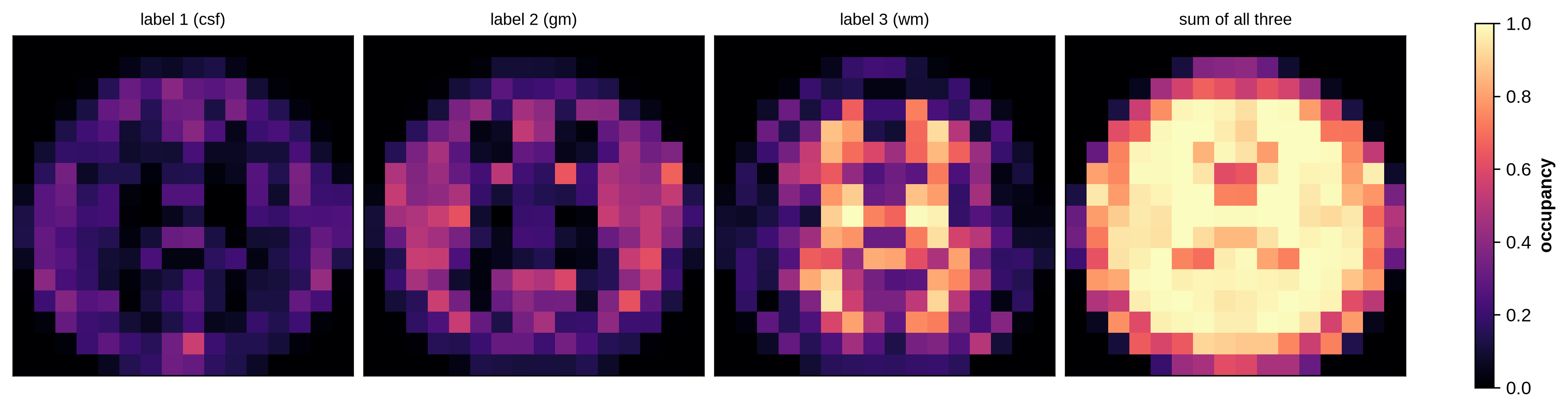
Does it survive an oblique grid?
Nothing above assumed axis alignment, but the fixture happens to be axis-aligned, so obliquity needs its own check. Rotating the target affine by 20° must leave total volume unchanged — the brain does not shrink because the grid was tilted.
theta = np.deg2rad(20.0)
rotation = np.eye(4)
rotation[:2, :2] = [[np.cos(theta), -np.sin(theta)], [np.sin(theta), np.cos(theta)]]
oblique_affine = rotation @ A_target

pv_oblique = mask_occupancy(
    brain_mask, np.zeros(target.nii.shape), target_affine=oblique_affine, min_coverage=0.0
)
oblique_volume = float(pv_oblique.occupancy.sum()) * abs(np.linalg.det(oblique_affine[:3, :3]))
print(f"axis-aligned {volume_in / 1000:.2f} mL   oblique {oblique_volume / 1000:.2f} mL")
axis-aligned 2699.25 mL oblique 2682.57 mL
Does the axis-aligned fast path agree with the general path?
mask_occupancy takes a separable shortcut whenever mask -> target is diagonal -- which every
fixture above is, so pv_auto already went through it. _force_general_path is a private test
hook that reruns the same call through _splat_slab instead, so the two can be compared directly
rather than trusted on the strength of an offline prototype.
pv_auto_general = mask_occupancy(tissue_seg, target, min_coverage=0.0, _force_general_path=True)Looking at it
The point of all of the above is a map you can lay over the anatomy and believe:
The map only means something laid over the anatomy it came from. To do that honestly, the T1 slice has to be the one the MRSI slice actually sits on — found by mapping the target slice index back through the transform rather than guessed:
occ = pv.occupancy.sel(label="mask").values
k = occ.shape[2] // 2

# Which T1 slice does target slice k correspond to?
z_t1 = int(
    round(
        affines.apply_affine(mask_from_tgt, [target.nii.shape[0] / 2, target.nii.shape[1] / 2, k])[
            2
        ]
    )
)
print(f"target slice k={k}  ->  T1 slice z={z_t1}")

fig, axes = plt.subplots(1, 3, figsize=(11, 3.4), layout="constrained")

panel(axes[0], t1_data[:, :, z_t1], f"T1, z={z_t1}", cmap="gray")

panel(axes[1], t1_data[:, :, z_t1], f"occupancy over T1, k={k}", cmap="gray")
extent = (-0.5, t1_data.shape[0] - 0.5, -0.5, t1_data.shape[1] - 0.5)
h_occ = axes[1].imshow(
    np.ma.masked_invalid(occ[:, :, k]).T,
    origin="lower",
    cmap="magma",
    vmin=0,
    vmax=1,
    alpha=0.6,
    extent=extent,
    interpolation="nearest",
)
fig.colorbar(h_occ, ax=axes[1], fraction=0.046, label="occupancy")

h_cov = panel(
    axes[2], pv.coverage.values[:, :, k], f"coverage, k={k}", cmap="viridis", vmin=0, vmax=1
)
fig.colorbar(h_cov, ax=axes[2], fraction=0.046, label="coverage")
target slice k=8 -> T1 slice z=98
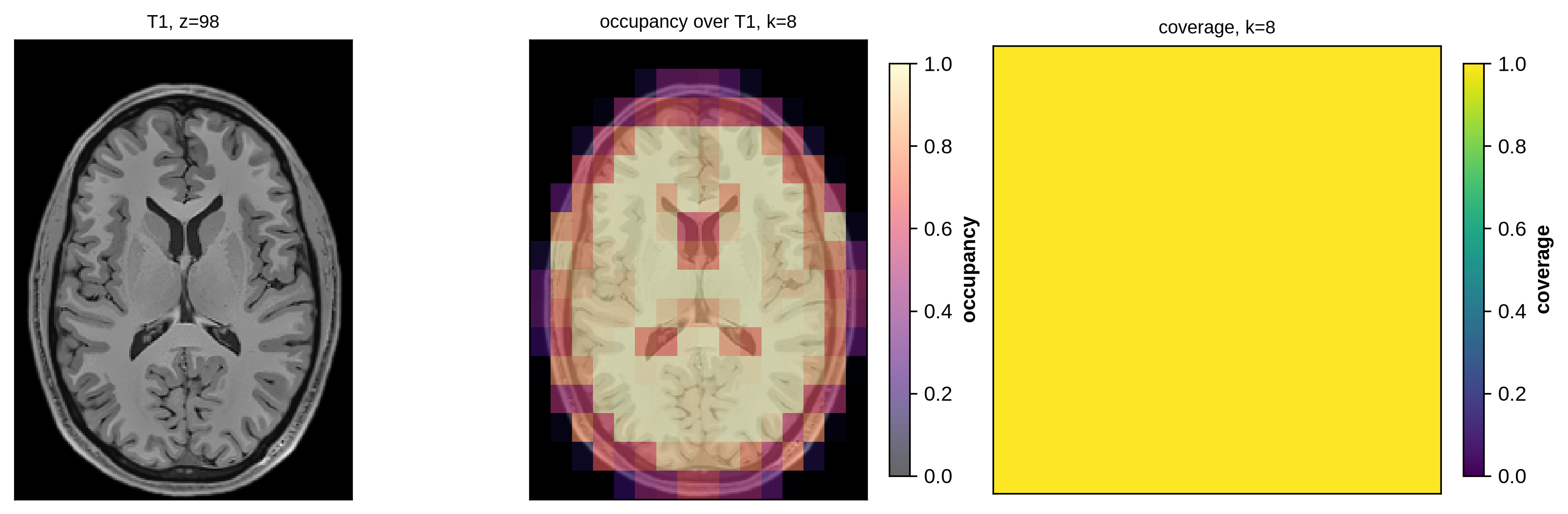
Occupancy falls off smoothly at the brain’s edge — those are the genuinely partial voxels, and their value is the fraction you would multiply a concentration by. The blanks in the middle panel are the NaNs: MRSI voxels the T1 never reached. Coverage, on the right, is flat at 1 across the interior and drops only where the MRSI grid runs past the T1 — which is exactly the red border from the lattice figure at the top of the page.